Sentinel-2 Field Delineation
Published:
🌍 The Mission
To engineer a robust field delineation pipeline capable of accurately identifying agricultural boundaries using high-resolution multi-channel satellite imagery provided by Solafune.
- The Challenge: The model had to resolve dense clusters of 100+ distinct farms within a single satellite patch, requiring high instance separation capabilities.
🌿 Spectral Feature Engineering
To augment the raw satellite bands, I computed pixel-wise spectral indices to feed the model explicit physical properties of the terrain. This “physics-informed” approach significantly improved boundary detection:
- NDVI (Normalized Difference Vegetation Index): * Bands: B8 (NIR) & B4 (Red).
- Purpose: Highlights the density of Green Vegetation, crucial for separating crops from soil.
- NDWI (Normalized Difference Water Index):
- Bands: B4 (Red) & B11 (SWIR).
- Purpose: Detects Surface Water, helping to distinguish irrigation channels from fields.
- NDSI (Normalized Difference Snow Index):
- Bands: B3 (Green) & B11 (SWIR).
- Purpose: Maps the extent of Snow Cover (or highly reflective surfaces) to prevent false positives.
- GSI (Grain Size Index):
- Bands: B4 (Red), B2 (Blue), & B3 (Green).
- Purpose: Identifies areas with advanced Desertification, aiding in the exclusion of non-arable land.
🛰️ Architecture & Backbones
Implemented and benchmarked a diverse suite of semantic segmentation models to maximize feature extraction:
- Unet: The standard baseline for biomedical and satellite segmentation.
- Unet++: Utilized nested dense skip pathways to reduce the semantic gap.
- FPN (Feature Pyramid Networks): Implemented to handle multi-scale detection across varying resolutions.
- DeepLabv3: Leveraged atrous (dilated) convolutions to capture wider context without losing spatial resolution.
📐 Mathematical Framework: Loss & Metrics
To handle the class imbalance between field boundaries and land area, I engineered a Joint Total Loss function:
1. The Objective Function \(L_{Total} = 0.9 \times L_{Focal} + 0.1 \times L_{Jaccard}\)
2. Focal Loss ($L_{Focal}$) Focuses learning on “hard” examples (sparse boundaries) by down-weighting easy negatives: \(L_{Focal}(p_t) = - (1 - p_t)^\gamma \log(p_t)\)
3. Jaccard Loss ($L_{Jaccard}$) & IoU Directly optimizes the Intersection over Union metric: \(IoU = \frac{|Y \cap \hat{Y}|}{|Y \cup \hat{Y}|} \quad \Rightarrow \quad L_{Jaccard} = 1 - IoU\)
⚙️ The Pipeline
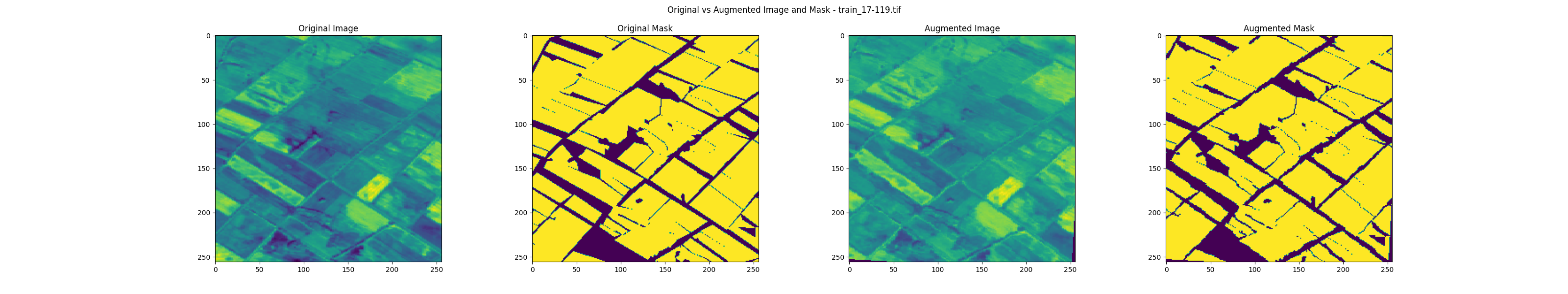
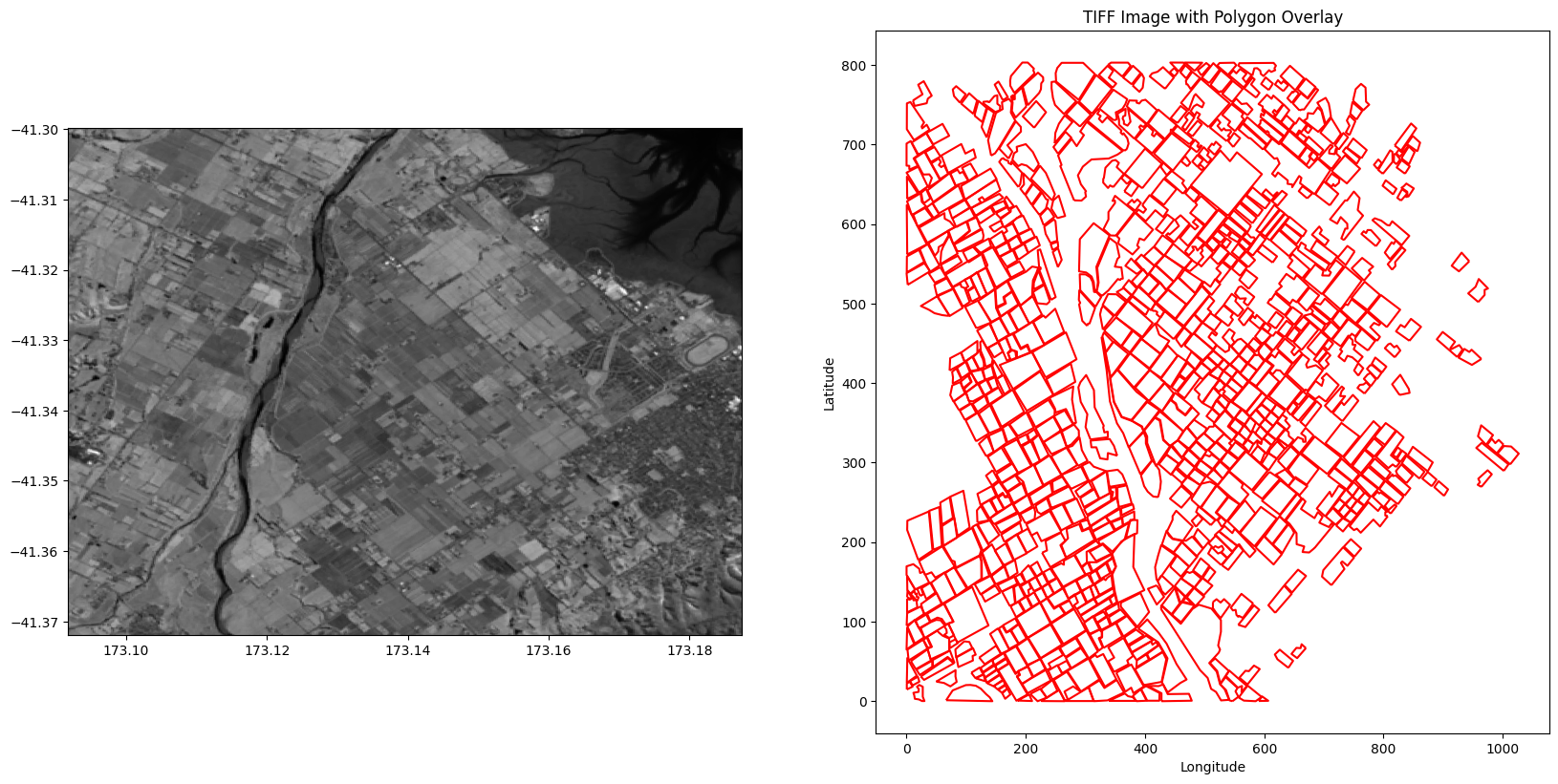
- Data Prep: Precise annotation polygons were extracted from raw satellite patches using OpenCV.
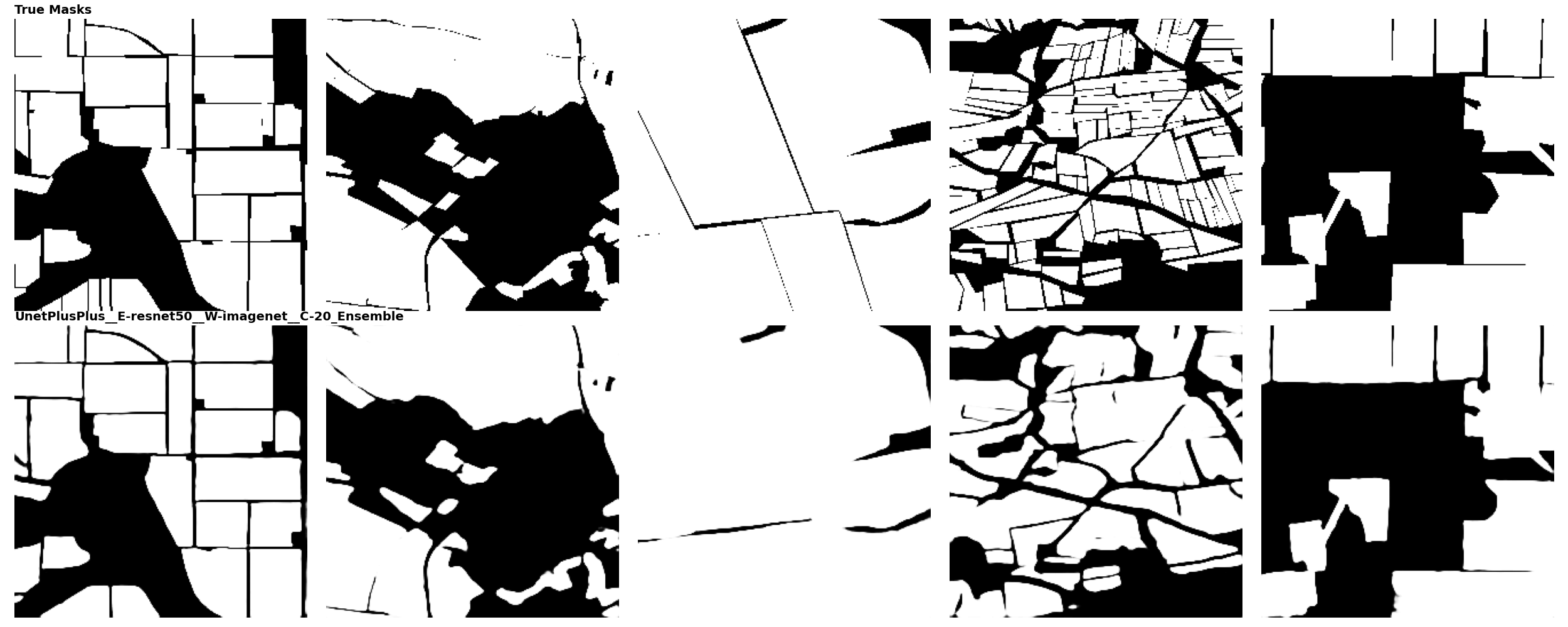
- Ensemble Strategy: Designed a stacking ensemble that aggregated prediction masks from the fine-tuned models. This “wisdom of crowds” approach smoothed out edge-case errors.
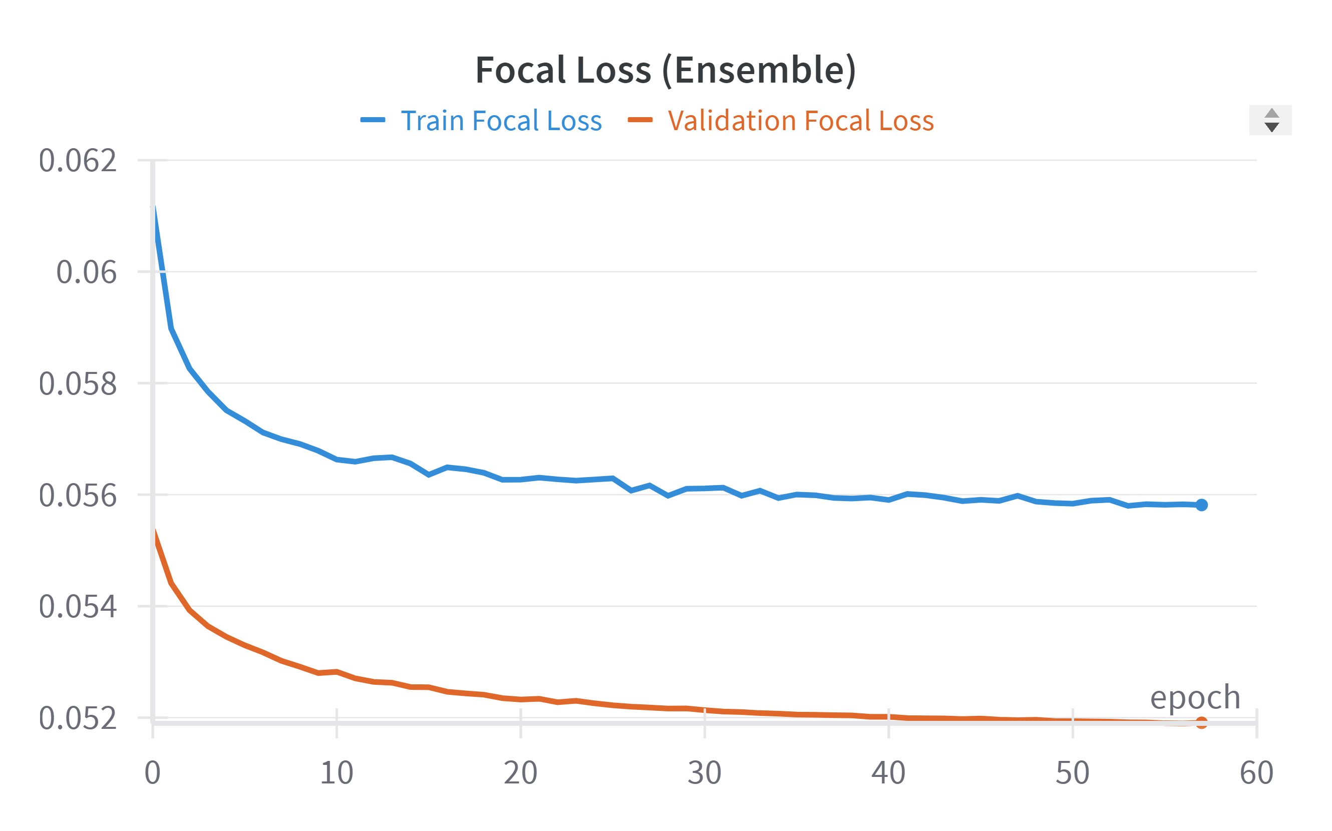
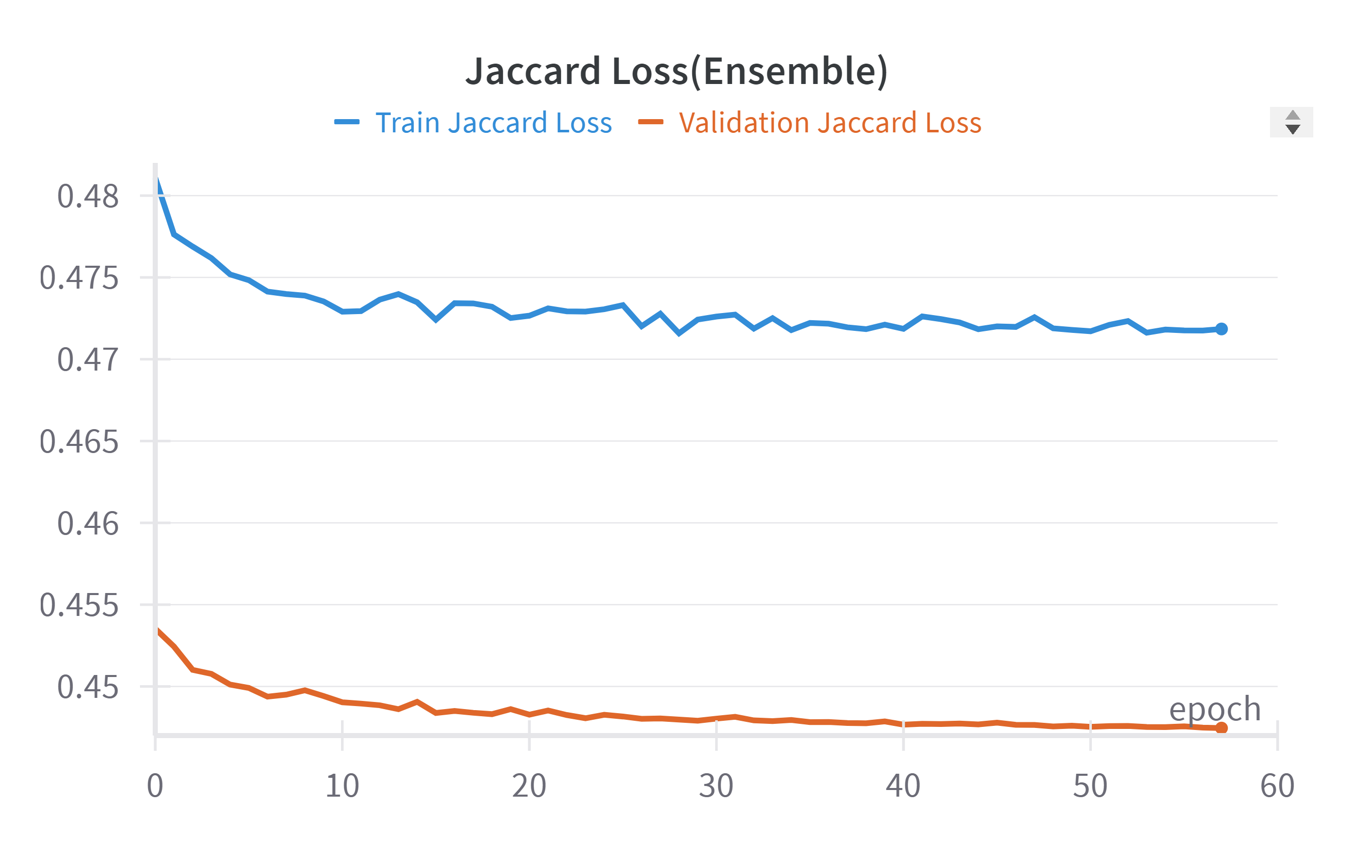
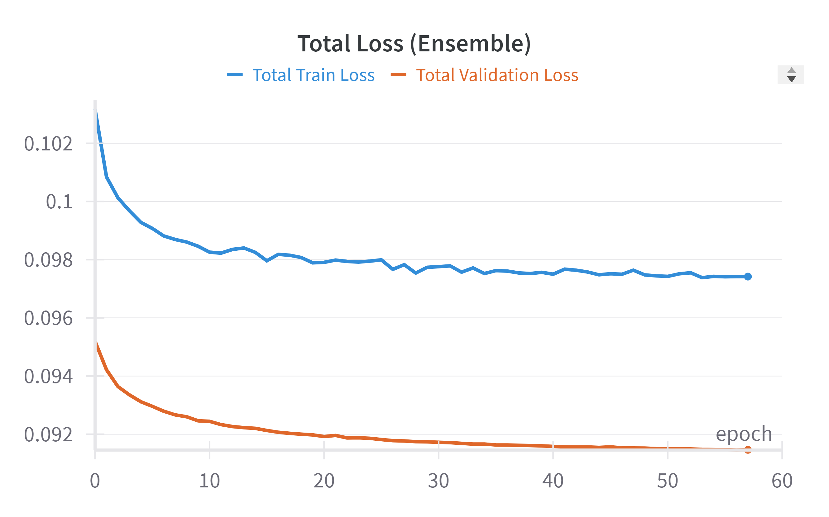
📉 Training Dynamics
The ensemble model demonstrated excellent convergence with strong generalization.
- Final Validation Focal Loss: Converged to 0.052.
- Final Validation Jaccard Loss: Stabilized at 0.447.
- Total Validation Loss: Achieved a final value of 0.091.
🎯 Impact
- Metric: Achieved a segmentation Intersection over Union (IoU) of 0.96.
- Result: Created a high-fidelity mapping tool suitable for automated agricultural analysis.
🔗 Links
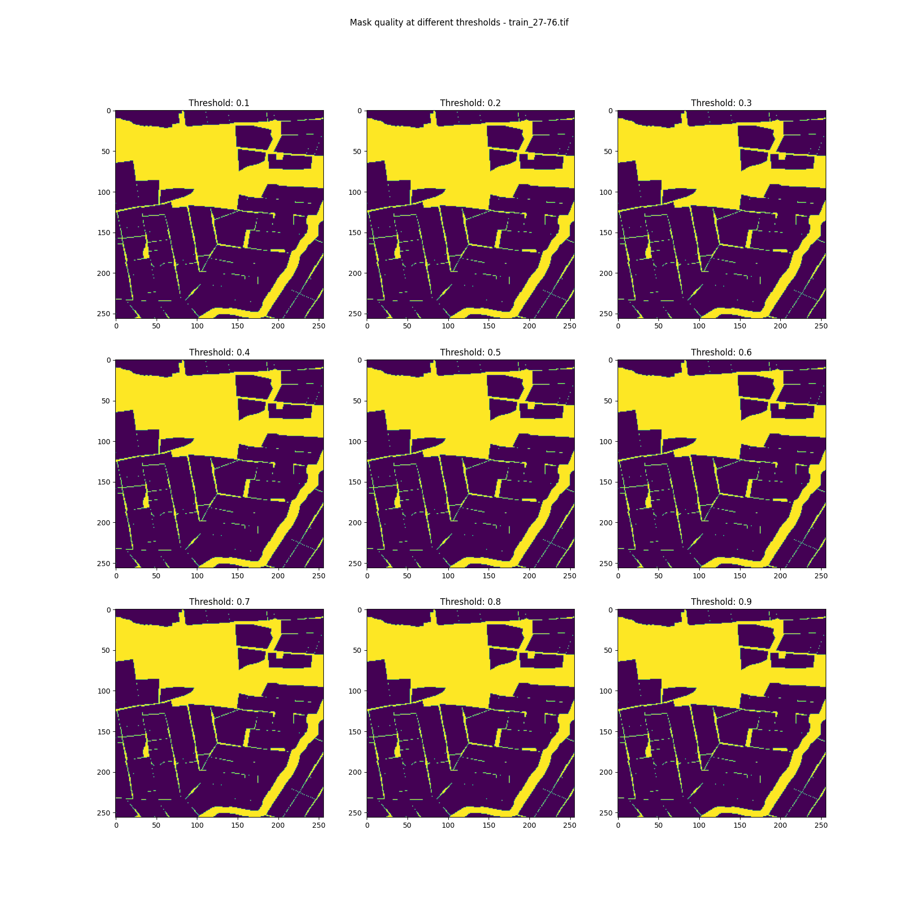
📸 Visual Library
Segmentation masks, satellite patches, and Training Loss curves.